1.配置环境(AutoDl)

https://mp.csdn.net/mp_blog/creation/editor/new/128688185

2.预备知识

2.1. 数据操作

import torch
print(torch.__version__) #1.2.0
#2.1.1入门
x=torch.arange(12)
print(x)
print(x.shape)
print(x.numel())#元素总数
X=x.reshape(3,4)
print(X)
#
print(torch.zeros(2,3,4))
print(torch.ones(2,3,4))
print(torch.randn(3,4))#均值为0，标准差为1
print(torch.tensor([[2,1,4,3],[1,2,3,4],[4,3,2,1]]))

#2.1.2运算符
x=torch.tensor([1,2,4,8],dtype=torch.float)
y=torch.tensor([2,2,2,2],dtype=torch.float)
print(x*y)#x-y,x*y,x/y(对应元素)
print(torch.exp(x))#原因: torch.exp()操作不支持Long类型的张量作为输入 解决方法: 将张量转为浮点型即可, 执行X=torch.arange(12,dtype=torch.float32).reshape(3,4)
Y=torch.tensor([[2.0,1,4,3],[1,2,3,4],[4,3,2,1]])
print(torch.cat((X,Y),dim=1))#dim=1
print(X==Y)

#2.1.3广播机制
a=torch.arange(3).reshape(3,1)
b=torch.arange(2).reshape(1,2)
print(a+b)

#2.1.4索引和切片
X=torch.arange(12,dtype=torch.float32).reshape(3,4)
print(X[-1],X[1:3])
X[1,2]=9#（1，2）处
print(X)
X[0:2,:]=12 #前两行
print(X)import numpy as np
Z = np.zeros_like(X)
print(Z)

#2.1.5节省内存(原地更新)
X=torch.arange(12,dtype=torch.float32).reshape(3,4)
Y=torch.tensor([[2.0,1,4,3],[1,2,3,4],[4,3,2,1]])
before=id(Y) #运行一些操作可能会导致为新结果分配内存
Y=Y+X
print(id(Y)==before)#首先，我们不想总是不必要地分配内存
#其次，如果我们不原地更新，其他引用仍然会指向旧的内存位置
#方式一：
print('id(Y):', id(Y))
Y[:] = X + Y
print('id(Y):', id(Y))#方式二
print('id(X):', id(X))
X[:]=X+Y
print('id(X):', id(X))
X+=Y
print('id(X):', id(X))

#2.1.6转换为其他Python对象
X=torch.arange(12,dtype=torch.float32).reshape(3,4)
A=X.numpy()
B=torch.tensor(A)
print(type(A),type(B))a=torch.tensor([3.5])
print(a,a.item(),float(a),int(a))#张量->标量

2.2. 数据预处理

#2.2.1 读取数据集
import os
os.makedirs(os.path.join('..','data'),exist_ok=True)
data_file=os.path.join('..','data','house_tiny.csv')
with open(data_file,'w') as f:f.write('NumRooms,Alley,Price\n')  # 列名f.write('NA,Pave,127500\n')  # 每行表示一个数据样本f.write('2,NA,106000\n')f.write('4,NA,178100\n')f.write('NA,NA,140000\n')import pandas as pd
data=pd.read_csv(data_file)
print(data)#2.2.2. 处理缺失值
inputs,outputs=data.iloc[:,0:2],data.iloc[:,2]
inputs=inputs.fillna(inputs.mean())#用同一列的均值替换“NaN”项
print(inputs)
#对于inputs中的类别值或离散值，我们将“NaN”视为一个类别。 由于“巷子类型”（“Alley”）列只接受两种类型的类别值“Pave”和“NaN”，
# pandas可以自动将此列转换为两列“Alley_Pave”和“Alley_nan”。
inputs=pd.get_dummies(inputs,dummy_na=True)
print(inputs)#2.2.3. 转换为张量格式
X,y=torch.tensor(inputs.values),torch.tensor(outputs.values)
print(X,y)

2.3. 线性代数

#2.3.1. 标量
x = torch.tensor(3.0)
y = torch.tensor(2.0)
#x + y, x * y, x / y, x**y#2.3.2. 向量以及长度、维度和形状
x = torch.arange(4)
print(x[3])
print(len(x))
print(x.shape)#2.3.3. 矩阵
A = torch.arange(20).reshape(5, 4)
print(A.T)#矩阵的转置
B = torch.tensor([[1, 2, 3], [2, 0, 4], [3, 4, 5]])
print(B == B.T)#2.3.4. 张量:向量是一阶张量，矩阵是二阶张量。
X = torch.arange(24).reshape(2, 3, 4)#2.3.5. 张量算法的基本性质
A = torch.arange(20, dtype=torch.float32).reshape(5, 4)
B = A.clone()  # 通过分配新内存，将A的一个副本分配给B
#A, A + B
print(A * B)#按元素的乘法a = 2
print(a + X)#(a * X).shape#2.3.6. 降维
x = torch.arange(4, dtype=torch.float32)
A = torch.arange(20, dtype=torch.float32).reshape(5, 4)
print(x.sum(),A.sum())#任意形状张量的元素和A_sum_axis0 = A.sum(axis=0)#通过求和所有行的元素来降维（轴0）
A_sum_axis1 = A.sum(axis=1)
#沿着行和列对矩阵求和，等价于对矩阵的所有元素进行求和。
A.sum(axis=[0, 1])  # 结果和A.sum()相同
# 2.3.6.1. 非降维求和
A = torch.arange(20, dtype=torch.float32).reshape(5, 4)
print(A)
sum_A = A.sum(axis=1, keepdims=True)
print(sum_A)
print(A / sum_A)#Broadcast
print(A.cumsum(axis=0)) #沿某个轴计算A元素的累积总和， 比如axis=0（按一行一行累计计算）#2.3.7. 点积（Dot Product）：相同位置的按元素乘积的和
x = torch.arange(4, dtype=torch.float32)
y = torch.ones(4, dtype = torch.float32)
print(torch.dot(x, y))
print(torch.dot(x, y)==torch.sum(x * y))#2.3.8. 矩阵向量积:=>向量
A = torch.arange(20, dtype=torch.float32).reshape(5, 4)
x = torch.arange(4, dtype=torch.float32)
print(A,x)
z=torch.mv(A, x)# 注意，A的列维数（沿轴1的长度）必须与x的维数（其长度）相同。
print(z)#[m,n]*[n]->[m]
print(A.shape)
print(x.shape)
print(z.shape)#2.3.9. 矩阵矩阵乘法
A = torch.arange(20, dtype=torch.float32).reshape(5, 4)
B = torch.ones(4, 3)
z=torch.mm(A, B)
print(z)
print(z.shape)#2.3.10. 范数:将向量映射到标量
#L2范数:向量元素平方和的平方根
#L1范数：向量元素的绝对值之和
#F范数:是矩阵元素平方和的平方根（L2）
u = torch.tensor([3.0, -4.0])
print(torch.norm(u))
print(torch.abs(u).sum())
print(torch.norm(torch.ones((4, 9))))
#2.3.10.1. 范数和目标
#在深度学习中，我们经常试图解决优化问题： 最大化分配给观测数据的概率; 最小化预测和真实观测之间的距离。

2.4. 微积分

#2.4.1. 导数和微分
import numpy as np
from d2l import torch as d2ldef f(x):return 3*x**2-4*x #导数：6x-4
def numerical_lim(f,x,h):return (f(x+h)-f(x))/hh=0.1
for i in range(5):print(f'h={h:.5f},numerical limit={numerical_lim(f,1,h):.5f}')h *=0.1x=np.arange(0,3,0.1)
d2l.plot(x,[f(x),2*x-3],'x','f(x)',legend=['f(x)','Target f(x) x=1'])
d2l.plt.show()#2.4.2. 偏导数
#2.4.3. 梯度
#2.4.4. 链式法则

2.5. 自动微分

import torch
print(torch.__version__) #1.2.0
#2.5.1. 一个简单的例子（标量变量）
#1)定义函数
x=torch.arange(4.0,requires_grad=True)
print(x.grad)  # 默认值是None
y = 2 * torch.dot(x, x)
#2）反向传播
y.backward()
#3）计算梯度
print(x.grad)
print(x.grad == 4 * x)#2.5.2. 非标量变量的反向传播
# 0）清楚累计梯度（注意：在默认情况下，PyTorch会累积梯度，再次计算梯度时，我们需要清除之前的值）
x.grad.zero_()
#1)定义函数
y=x*x
#2）反向传播
#对非标量调用backward需要传入一个gradient参数，该参数指定微分函数关于self的梯度
#等价于y.backward(torch.ones(len(x)))
#等价于y.backward(torch.ones_like(x), retain_graph=True)
y.sum().backward()
#3）计算梯度
print(x.grad)#2.5.3. 分离计算：将某些计算移动到记录的计算图之外
x.grad.zero_()
y = x * x
y.sum().backward()
print(x.grad == 2 * x)###
x.grad.zero_()
u = y.detach()#这里分离y来返回一个新变量u，该变量与y具有相同的值， 但丢弃计算图中如何计算y的任何信息。换句话说，梯度不会向后流经u到x。
#注意：计算图是从下面开始，将u作为常数处理
z = u * x
z.sum().backward()#因此，下面的反向传播函数计算z=u*x关于x的偏导数，同时将u作为常数处理， 而不是z=x*x*x关于x的偏导数
print(x.grad == u)#2.5.4. Python控制流的梯度计算
def f(a): #相当于f(a)=Kab = a * 2while b.norm() < 1000:b = b * 2if b.sum() > 0:c = belse:c = 100 * breturn c
a=torch.randn(size=(),requires_grad=True)
y=f(a)
y.backward()
print(a.grad==y/a)

2.6. 概率

import torch
print(torch.__version__) #1.2.0
#2.6.1. 基本概率论
from torch.distributions import multinomial
from d2l import torch as d2l#大数定理：概率如何随着时间的推移收敛到真实概率。
# 让我们进行500组实验，每组抽取10个样本。
fair_probs = torch.ones([6]) / 6  #1)为了抽取一个样本，即掷骰子，传入一个概率向量
counts = multinomial.Multinomial(10, fair_probs).sample((500,)) #2)输出是另一个相同长度的向量：它在索引i处的值是第j次采样结果中出现的次数
cum_counts = counts.cumsum(dim=0) #例如：tensor([[  0.,   2.,   1.,   4.,   2.,   1.],[  2.,   3.,   3.,   6.,   3.,   3.],,,,]
#cum_counts.sum(dim=1, keepdims=True) [[10],[20]]
estimates = cum_counts / cum_counts.sum(dim=1, keepdims=True)# 相对频率作为估计值#区别
# cumsum(dim=0/1)做一行一行或一列一列累加，维度相比于之前不变
# sum(dim=0/1) 沿某一轴累加，维度相比于之前变化（keepdims=True会不变）
#[[1,2,3],[2,3,4]]
#cumsum(dim=0):[[1,2,3],[3,5,7]]
#sum(dim=0):[[3,5,7]]d2l.set_figsize((6, 4.5))
for i in range(6):d2l.plt.plot(estimates[:, i].numpy(),label=("P(i=" + str(i + 1) + ")"))
d2l.plt.axhline(y=0.167, color='black', linestyle='dashed')
d2l.plt.gca().set_xlabel('Groups of experiments')
d2l.plt.gca().set_ylabel('Estimated probability')
d2l.plt.legend()
d2l.plt.show()

2.6.2.6. 应用：
https://zh-v2.d2l.ai/chapter_preliminaries/probability.html

2.7. 查阅文档

#2.7.1. 查找模块中的所有函数和类
import torch
print(dir(torch.distributions))#2.7.2. 查找特定函数和类的用法
help(torch.ones)

3.线性神经网络

回归问题（值回归）

3.1.线性回归

#3.1.2. 矢量化加速
import torch
from d2l import torch as d2ln = 10000
a = torch.ones([n])
b = torch.ones([n])
#方式一：for-loop
c = torch.zeros(n)
timer = d2l.Timer()
for i in range(n):c[i] = a[i] + b[i]
print(f'{timer.stop():.5f} sec')#方式二:使用重载的+运算符(矢量化加速)
timer.start()
d = a + b
print(f'{timer.stop():.5f} sec')#3.1.3. 正态分布与平方损失
import math
import numpy as np
def normal(x, mu, sigma):p = 1 / math.sqrt(2 * math.pi * sigma**2)return p * np.exp(-0.5 / sigma**2 * (x - mu)**2)# 再次使用numpy进行可视化
x = np.arange(-7, 7, 0.01)# 均值和标准差对
params = [(0, 1), (0, 2), (3, 1)]
d2l.plot(x, [normal(x, mu, sigma) for mu, sigma in params], xlabel='x',ylabel='p(x)', figsize=(4.5, 2.5),legend=[f'mean {mu}, std {sigma}' for mu, sigma in params])
d2l.plt.show()

3.2. 线性回归的从零开始实现

import random
import torch
from d2l import torch as d2l
#3.2.1. 生成数据集
def synthetic_data(w, b, num_examples):  #@save"""生成y=Xw+b+噪声"""#featureX = torch.normal(0, 1, (num_examples, len(w)))#行：num_examples 列：len(w)#label(含 noise)y = torch.matmul(X, w) + b #行：num_examples 列：1y += torch.normal(0, 0.01, y.shape) #+噪声return X, y.reshape((-1, 1))#标量->一维张量true_w = torch.tensor([2, -3.4])
true_b = 4.2
features, labels = synthetic_data(true_w, true_b, 1000)
#print('features:', features[0],'\nlabel:', labels[0])d2l.set_figsize()
d2l.plt.scatter(features[:, 1].detach().numpy(), labels.detach().numpy(), 1) #从计算图中detach出来，再转numpy
#d2l.plt.show()#3.2.2. 读取数据集
def data_iter(batch_size, features, labels):num_examples = len(features)indices = list(range(num_examples))#索引[0,```,999]# 这些样本是随机读取的，没有特定的顺序（通过随机打乱索引实现）random.shuffle(indices)for i in range(0, num_examples, batch_size):#范围：[0, num_examples),步长：batch_sizebatch_indices = torch.tensor(indices[i: min(i + batch_size, num_examples)])yield features[batch_indices], labels[batch_indices] #每次loop,生成batch_size个features和labels#batch_size = 10
# for X, y in data_iter(batch_size, features, labels):
#     print(X, '\n', y) #这里打印一次：即batch_size个features和labels
#     break#3.2.4. 定义模型
def linreg(X, w, b):  #@save"""线性回归模型"""return torch.matmul(X, w) + b #Broadcast#3.2.3. 初始化模型参数
w = torch.normal(0, 0.01, size=(2,1), requires_grad=True)
b = torch.zeros(1, requires_grad=True)#3.2.5. 定义损失函数
def squared_loss(y_hat, y):  #@save"""均方损失"""return (y_hat - y.reshape(y_hat.shape)) ** 2 / 2 #shape：(batch_size,1)#3.2.6. 定义优化算法
#这里params=[w,b]
def sgd(params, lr, batch_size):  #@save"""小批量随机梯度下降"""with torch.no_grad(): #更新时，不参与梯度计算for param in params:param -= lr * param.grad / batch_size #/batch_size:因为loss是以bach_size计算的param.grad.zero_()#3.2.7. 训练
num_epochs = 3
batch_size = 10
lr = 0.03net = linreg #model
loss = squared_loss #targetfor epoch in range(num_epochs):#1）按batch更新：batch_size个feature为一组，一共num_examples/batch_size组for X, y in data_iter(batch_size, features, labels):l = loss(net(X, w, b), y)  # 2)X和y的小批量损失# 因为l形状是(batch_size,1)，而不是一个标量。l中的所有元素被加到一起，# 并以此计算关于[w,b]的梯度l.sum().backward()sgd([w, b], lr, batch_size)  #3)使用参数的梯度更新参数with torch.no_grad():train_l = loss(net(features, w, b), labels)#4)这里的w, b为该epoch的最后一次更新值print(f'epoch {epoch + 1}, loss {float(train_l.mean()):f}')print(f'w的估计误差: {true_w - w.reshape(true_w.shape)}')
print(f'b的估计误差: {true_b - b}')

3.3. 线性回归的简洁实现

import numpy as np
import torch
from torch.utils import data
from d2l import torch as d2l#3.2.1. 生成数据集
true_w = torch.tensor([2, -3.4])
true_b = 4.2
features, labels = d2l.synthetic_data(true_w, true_b, 1000)#3.2.2. 读取数据集（key）
def load_array(data_arrays, batch_size, is_train=True):  #@save"""构造一个PyTorch数据迭代器"""dataset = data.TensorDataset(*data_arrays)return data.DataLoader(dataset, batch_size, shuffle=is_train)batch_size = 10
data_iter = load_array((features, labels), batch_size)
#print(next(iter(data_iter))) #使用iter构造Python迭代器，并使用next从迭代器中获取第一项#3.2.4. 定义模型
# nn是神经网络的缩写
from torch import nn
##Sequential类可以将多个层串联在一起
net = nn.Sequential(nn.Linear(2, 1)) #第一个指定输入特征形状，即2，第二个指定输出特征形状，输出特征形状为单个标量，因此为1。#3.2.3. 初始化模型参数
#使用替换方法normal_和fill_来重写参数值
net[0].weight.data.normal_(0, 0.01)
net[0].bias.data.fill_(0)#3.2.5. 定义损失函数
loss = nn.MSELoss()#默认情况下，它返回所有样本损失的平均值#3.2.6. 定义优化算法
#指定优化的参数 （可通过net.parameters()从我们的模型中获得）以及优化算法所需的超参数字典
trainer = torch.optim.SGD(net.parameters(), lr=0.03)#3.2.7. 训练
num_epochs = 3
for epoch in range(num_epochs):for X, y in data_iter:#1）每次一个batch_sizel = loss(net(X) ,y)trainer.zero_grad()  # 必须在l.backward()前面，否则梯度累计l.backward()trainer.step()#2）验收该epoch更新的效果l = loss(net(features), labels)print(f'epoch {epoch + 1}, loss {l:f}')#验证最后的更新好的model
w = net[0].weight.data
print('w的估计误差：', true_w - w.reshape(true_w.shape))
b = net[0].bias.data
print('b的估计误差：', true_b - b)

分类问题（概率回归）

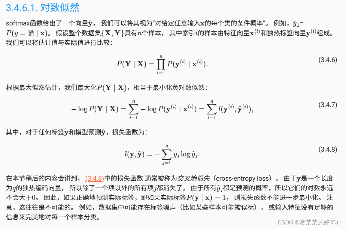
3.4. softmax回归：

softmax：获取一个向量并将其映射为概率（输出类别的概率分布）
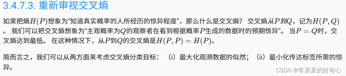
交叉熵损失（cross-entropy loss）：衡量两个概率分布之间差异

3.5. 图像分类数据集

import torch
import torchvision
from torch.utils import data
from torchvision import transforms
from d2l import torch as d2ld2l.use_svg_display()# 3.5.1. 读取数据集
# 通过ToTensor实例将图像数据从PIL类型变换成32位浮点数格式，
# 并除以255使得所有像素的数值均在0～1之间
trans = [transforms.ToTensor()]
trans = transforms.Compose(trans)
mnist_train = torchvision.datasets.FashionMNIST(root="./data", train=True, transform=trans, download=False)#True
mnist_test = torchvision.datasets.FashionMNIST(root="./data", train=False, transform=trans, download=False)#数据集情况
print(len(mnist_train), len(mnist_test))
print(mnist_train[0][0].shape)  # 每个输入图像的高度和宽度均为28像素,灰度图def get_fashion_mnist_labels(labels):  #@save"""返回Fashion-MNIST数据集的文本标签"""text_labels = ['t-shirt', 'trouser', 'pullover', 'dress', 'coat','sandal', 'shirt', 'sneaker', 'bag', 'ankle boot']return [text_labels[int(i)] for i in labels]def show_images(imgs, num_rows, num_cols, titles=None, scale=1.5):  #@save"""绘制图像列表"""figsize = (num_cols * scale, num_rows * scale)_, axes = d2l.plt.subplots(num_rows, num_cols, figsize=figsize)axes = axes.flatten()for i, (ax, img) in enumerate(zip(axes, imgs)):if torch.is_tensor(img):# 图片张量ax.imshow(img.numpy())else:# PIL图片ax.imshow(img)ax.axes.get_xaxis().set_visible(False)ax.axes.get_yaxis().set_visible(False)if titles:ax.set_title(titles[i])return axes
#batch个数据可视化
X, y = next(iter(data.DataLoader(mnist_train,batch_size=18)))  # 拿第一个batch数据,例如y=tensor([9, 0, 0, 3, 0, 2, 7, 2, 5, 5, 0, 9, 5, 5, 7, 9, 1, 0])
show_images(X.reshape(18, 28, 28), 2, 9, titles=get_fashion_mnist_labels(y))
d2l.plt.show()#3.5.3. 整合所有组件(key)
def get_dataloader_workers():  #@save"""使用4个进程来读取数据"""return 4def load_data_fashion_mnist(batch_size, resize=None):  #@save #注意：这里resize的作用可以迎合各种模型的输入要求"""下载Fashion-MNIST数据集，然后将其加载到内存中"""# 3.5.1. 读取数据集# 通过ToTensor实例将图像数据从PIL类型变换成32位浮点数格式，# 并除以255使得所有像素的数值均在0～1之间trans = [transforms.ToTensor()]if resize:trans.insert(0, transforms.Resize(resize))trans = transforms.Compose(trans)mnist_train = torchvision.datasets.FashionMNIST(root="./data", train=True, transform=trans, download=False)#Truemnist_test = torchvision.datasets.FashionMNIST(root="./data", train=False, transform=trans, download=False)return (data.DataLoader(mnist_train, batch_size, shuffle=True,num_workers=get_dataloader_workers()),data.DataLoader(mnist_test, batch_size, shuffle=False,num_workers=get_dataloader_workers()))train_iter, test_iter = load_data_fashion_mnist(32, resize=64)#3.5.2. 按小批量方式读取全部数据
timer = d2l.Timer()
for X, y in train_iter:print(X.shape, X.dtype, y.shape, y.dtype)#torch.Size([32, 1, 64, 64]) torch.float32 torch.Size([32]) torch.int64break #这里只显示一个batch_size的数据
print(f'使用4个进程来读取数据：{4},time:{timer.stop():.2f} sec')

3.6. softmax回归的从零开始实现

import torch
from IPython import display
from d2l import torch as d2limport torchvision
from torch.utils import data
from torchvision import transformsclass Accumulator:  # @save"""在n个变量上累加"""def __init__(self, n):self.data = [0.0] * ndef add(self, *args):self.data = [a + float(b) for a, b in zip(self.data, args)]def reset(self):self.data = [0.0] * len(self.data)def __getitem__(self, idx):return self.data[idx]class Animator:  # @save"""在动画中绘制数据"""def __init__(self, xlabel=None, ylabel=None, legend=None, xlim=None,ylim=None, xscale='linear', yscale='linear',fmts=('-', 'm--', 'g-.', 'r:'), nrows=1, ncols=1,figsize=(3.5, 2.5)):# 增量地绘制多条线if legend is None:legend = []d2l.use_svg_display()self.fig, self.axes = d2l.plt.subplots(nrows, ncols, figsize=figsize)if nrows * ncols == 1:self.axes = [self.axes, ]# 使用lambda函数捕获参数self.config_axes = lambda: d2l.set_axes(self.axes[0], xlabel, ylabel, xlim, ylim, xscale, yscale, legend)self.X, self.Y, self.fmts = None, None, fmtsdef add(self, x, y):# 向图表中添加多个数据点if not hasattr(y, "__len__"):y = [y]n = len(y)if not hasattr(x, "__len__"):x = [x] * nif not self.X:self.X = [[] for _ in range(n)]if not self.Y:self.Y = [[] for _ in range(n)]for i, (a, b) in enumerate(zip(x, y)):if a is not None and b is not None:self.X[i].append(a)self.Y[i].append(b)self.axes[0].cla()for x, y, fmt in zip(self.X, self.Y, self.fmts):self.axes[0].plot(x, y, fmt)self.config_axes()display.display(self.fig)display.clear_output(wait=True)#bug:
#1，修改进程数：将DataLoader中的num_workers=2,改成num_workers=0,仅执行主进程。运行成功！！！
#2,使用多进程习惯用法：再for循环前加上main函数，成功运行！！！
if __name__ == '__main__':#1. 读取数据集def get_dataloader_workers():  # @save"""使用4个进程来读取数据"""return 4def load_data_fashion_mnist(batch_size, resize=None):  # @save #注意：这里resize的作用可以迎合各种模型的输入要求"""下载Fashion-MNIST数据集，然后将其加载到内存中"""# 3.5.1. 读取数据集# 通过ToTensor实例将图像数据从PIL类型变换成32位浮点数格式，# 并除以255使得所有像素的数值均在0～1之间trans = [transforms.ToTensor()]if resize:trans.insert(0, transforms.Resize(resize))trans = transforms.Compose(trans)mnist_train = torchvision.datasets.FashionMNIST(root="./data", train=True, transform=trans, download=False)  # Truemnist_test = torchvision.datasets.FashionMNIST(root="./data", train=False, transform=trans, download=False)return (data.DataLoader(mnist_train, batch_size, shuffle=True,num_workers=get_dataloader_workers()),data.DataLoader(mnist_test, batch_size, shuffle=False,num_workers=get_dataloader_workers()))batch_size = 256train_iter, test_iter = load_data_fashion_mnist(batch_size) #将全部样本，按batch_size分组#3.6.1. 初始化模型参数num_inputs = 784 #输入时，将图像展平：1x28x28(神经元)num_outputs = 10 #输出类别数：10W = torch.normal(0, 0.01, size=(num_inputs, num_outputs), requires_grad=True) #利用高斯随机初始化b = torch.zeros(num_outputs, requires_grad=True)# 3.6.2. 定义softmax操作def softmax(X):X_exp = torch.exp(X)partition = X_exp.sum(1, keepdim=True)#沿着y轴求和return X_exp / partition  # 这里应用了广播机制##X = torch.tensor([[1.0, 2.0, 3.0], [4.0, 5.0, 6.0]])# print(X.sum(0, keepdim=True), X.sum(1, keepdim=True))## X = torch.normal(0, 1, (2, 5))# X_prob = softmax(X)# print(X_prob, X_prob.sum(1))#3.6.3. 定义模型def net(X):return softmax(torch.matmul(X.reshape((-1, W.shape[0])), W) + b)#(-1, W.shape[0])：对输入的一个flatten：batch_size x 784(这是区别于线性模型的标志)#3.6.4. 定义损失函数def cross_entropy(y_hat, y):#key:如果真实类别为1，而索引为1对应的估计概率很小就会导致交叉熵损失很大#size:[batch_size]return - torch.log(y_hat[range(len(y_hat)), y]) #y_hat[range(len(y_hat)), y]:使用y作为y_hat中概率的索引(即拿到y对应类别的估计概率y_hat)# cross_entropy解释：使用y作为y_hat中概率的索引# y_hat = torch.tensor([[0.1, 0.3, 0.6], [0.3, 0.2, 0.5]])#表示两个样本各属于三种类的概率值# y = torch.tensor([0, 2]) #比如样本0真实属于0类，样本1真实属于2类# 比如，y_hat的[0]号样本[0.1, 0.3, 0.6]中取索引为y[0]的概率值，即样本0的属于0类的估计概率0.1# y_hat的[1]号样本[0.3, 0.2, 0.5]中取索引为y[1]的概率值，即样本1的属于2类的估计概率0.5# print(y_hat[[0, 1], y]) #tensor([0.1000, 0.5000])#print(cross_entropy(y_hat, y))#tensor([2.3026, 0.6931])，说明样本0的属于0类的估计误差大# 3.6.5. 分类精度def accuracy(y_hat, y):  # @save"""计算预测正确的数量"""#y_hat.shape：[batch_size,num_outputs]if len(y_hat.shape) > 1 and y_hat.shape[1] > 1: #说明维度大于1，且列数（即预测类别）也大于1y_hat = y_hat.argmax(axis=1) #选择预测概率最高的类(返回索引)cmp = y_hat.type(y.dtype) == y#步骤：1）统一数据类型：y_hat变成y的数据类型 2）y_hat与y的对应类别(索引)做比较(bool)return float(cmp.type(y.dtype).sum())#3）统计估计类别与实际类别(索引)一致的个数#print(accuracy(y_hat, y) / len(y))# 可以评估在任意模型net的精度def evaluate_accuracy(net, data_iter):  #@save"""计算在指定数据集上模型的精度"""if isinstance(net, torch.nn.Module):#说明net是torch.nn.Module实现的net.eval()  # 将模型设置为评估模式(不需要计算梯度，更新模型了)metric = Accumulator(2)  # metric[0]：正确预测数、metric[0]：预测总数with torch.no_grad():for X, y in data_iter:metric.add(accuracy(net(X), y), y.numel())#每次对应batch_size个样本return metric[0] / metric[1]print('模型的初始精度:',evaluate_accuracy(net, test_iter))#3.6.6. 训练def train_epoch_ch3(net, train_iter, loss, updater):  #@save"""训练模型一个迭代周期（定义见第3章）"""if isinstance(net, torch.nn.Module):#说明net是torch.nn.Module实现的net.train() # 将模型设置为训练模式(需要计算梯度，更新模型了)# metric[0]:训练损失总和、metric[1]:训练准确度总和、metric[2]:样本数metric = Accumulator(3)for X, y in train_iter:# 计算梯度并更新参数y_hat = net(X)l = loss(y_hat, y)if isinstance(updater, torch.optim.Optimizer):#说明updater是torch.optim.Optimizer实现的# 使用PyTorch内置的优化器和损失函数updater.zero_grad()l.mean().backward()updater.step()else:# 使用定制的优化器和损失函数l.sum().backward()updater(X.shape[0])#X.shape[0]:batch_sizemetric.add(float(l.sum()), accuracy(y_hat, y), y.numel())#每次对应batch_size个样本# 返回训练损失和训练精度(epoch)return metric[0] / metric[2], metric[1] / metric[2]###key-key-keydef train_ch3(net, train_iter, test_iter, loss, num_epochs, updater):  #@save"""训练模型（定义见第3章）"""animator = Animator(xlabel='epoch', xlim=[1, num_epochs], ylim=[0.3, 0.9],legend=['train loss', 'train acc', 'test acc'])for epoch in range(num_epochs):train_metrics = train_epoch_ch3(net, train_iter, loss, updater) #for 训练集表现test_acc = evaluate_accuracy(net, test_iter) #for 测试集表现animator.add(epoch + 1, train_metrics + (test_acc,)) #每epoch：实时显示训练精度，训练损失和测试精度train_loss, train_acc = train_metricsassert train_loss < 0.5, train_lossassert train_acc <= 1 and train_acc > 0.7, train_accassert test_acc <= 1 and test_acc > 0.7, test_acc#自定义的优化算法lr = 0.1def updater(batch_size):return d2l.sgd([W, b], lr, batch_size)num_epochs = 10train_ch3(net, train_iter, test_iter, cross_entropy, num_epochs, updater)d2l.plt.show()#3.6.7. 预测def predict_ch3(net, test_iter, n=6):  #@save"""预测标签（定义见第3章）"""for X, y in test_iter:break #这里只取一个batch样本trues = d2l.get_fashion_mnist_labels(y)preds = d2l.get_fashion_mnist_labels(net(X).argmax(axis=1))titles = [true +'\n' + pred for true, pred in zip(trues, preds)]d2l.show_images(X[0:n].reshape((n, 28, 28)), 1, n, titles=titles[0:n])predict_ch3(net, test_iter)d2l.plt.show()

3.7. softmax回归的简洁实现

import torch
from torch import nn
from d2l import torch as d2lbatch_size = 256
train_iter, test_iter = d2l.load_data_fashion_mnist(batch_size)#3.7.1. 初始化模型参数(key)
# PyTorch不会隐式地调整输入的形状。因此，
# 区别于简单线性回归模型：我们在线性层前定义了展平层（flatten），来调整网络输入的形状
net = nn.Sequential(nn.Flatten(), nn.Linear(784, 10)) #nn.Flatten()【变成 2D tensor】:第零维度保持，例如1x28x28->1x748def init_weights(m):if type(m) == nn.Linear: #Sequential->m->如果是线形层nn.init.normal_(m.weight, std=0.01) #->初始化权重net.apply(init_weights)#3.7.2. 重新审视Softmax的实现
#在交叉熵损失函数中传递未归一化的预测，并同时计算softmax及其对数
loss = nn.CrossEntropyLoss(reduction='none')#3.7.3. 优化算法
trainer = torch.optim.SGD(net.parameters(), lr=0.1)#3.7.4. 训练
num_epochs = 10
d2l.train_ch3(net, train_iter, test_iter, loss, num_epochs, trainer)
d2l.plt.show()

4.多层感知机

4.1.多层感知机

#隐藏层：任何像素的重要性取决于该像素的上下文（周围像素的值）
#激活函数：以防止多层感知机退化成线性模型

#4.1.2. 激活函数
import torch
from d2l import torch as d2l#4.1.2.1. ReLU函数
x = torch.arange(-8.0, 8.0, 0.1, requires_grad=True)
y = torch.relu(x)
d2l.plot(x.detach(), y.detach(), 'x', 'relu(x)', figsize=(5, 2.5))y.backward(torch.ones_like(x), retain_graph=True)#等价于#等价于y.backward(torch.ones(len(x))) <=> y.sum().backward()
d2l.plot(x.detach(), x.grad, 'x', 'grad of relu', figsize=(5, 2.5))#绘制ReLU函数的导数
d2l.plt.show()#4.1.2.2. sigmoid函数
y = torch.sigmoid(x)
d2l.plot(x.detach(), y.detach(), 'x', 'sigmoid(x)', figsize=(5, 2.5))x.grad.data.zero_()# 清除以前的梯度
y.backward(torch.ones_like(x),retain_graph=True)
d2l.plot(x.detach(), x.grad, 'x', 'grad of sigmoid', figsize=(5, 2.5))#4.1.2.3. tanh函数
y = torch.tanh(x)
d2l.plot(x.detach(), y.detach(), 'x', 'tanh(x)', figsize=(5, 2.5))x.grad.data.zero_()# 清除以前的梯度
y.backward(torch.ones_like(x),retain_graph=True)
d2l.plot(x.detach(), x.grad, 'x', 'grad of tanh', figsize=(5, 2.5))

4.2. 多层感知机的从零开始实现

import torch
from torch import nn
from d2l import torch as d2limport torchvision
from torch.utils import data
from torchvision import transforms
#bug:
#1，修改进程数：将DataLoader中的num_workers=2,改成num_workers=0,仅执行主进程。运行成功！！！
#2,使用多进程习惯用法：再for循环前加上main函数，成功运行！！！
def get_dataloader_workers():  # @save"""使用0个进程来读取数据"""return 0def load_data_fashion_mnist(batch_size, resize=None):  # @save #注意：这里resize的作用可以迎合各种模型的输入要求"""下载Fashion-MNIST数据集，然后将其加载到内存中"""# 3.5.1. 读取数据集# 通过ToTensor实例将图像数据从PIL类型变换成32位浮点数格式，# 并除以255使得所有像素的数值均在0～1之间trans = [transforms.ToTensor()]if resize:trans.insert(0, transforms.Resize(resize))trans = transforms.Compose(trans)mnist_train = torchvision.datasets.FashionMNIST(root="./data", train=True, transform=trans, download=False)  # Truemnist_test = torchvision.datasets.FashionMNIST(root="./data", train=False, transform=trans, download=False)return (data.DataLoader(mnist_train, batch_size, shuffle=True,num_workers=get_dataloader_workers()),data.DataLoader(mnist_test, batch_size, shuffle=False,num_workers=get_dataloader_workers()))batch_size = 256
train_iter, test_iter = load_data_fashion_mnist(batch_size)  # 将全部样本，按batch_size分组#4.2.1. 初始化模型参数
num_inputs, num_outputs, num_hiddens = 784, 10, 256W1 = nn.Parameter(torch.randn(num_inputs, num_hiddens, requires_grad=True) * 0.01)#nn.Parameter可加可不加
b1 = nn.Parameter(torch.zeros(num_hiddens, requires_grad=True))W2 = nn.Parameter(torch.randn(num_hiddens, num_outputs, requires_grad=True) * 0.01)
b2 = nn.Parameter(torch.zeros(num_outputs, requires_grad=True))params = [W1, b1, W2, b2]#4.2.2. 激活函数
def relu(X):a = torch.zeros_like(X)return torch.max(X, a) #ReLU(x)=max(0,x)#4.2.3. 模型
def net(X):X = X.reshape((-1, num_inputs)) #(-1, num_inputs)：batsize x num_inputs 256 X 784H = relu(X@W1 + b1)  # 这里“@”代表矩阵乘法return (H@W2 + b2)#4.2.4. 损失函数
loss = nn.CrossEntropyLoss(reduction='none')#4.2.5. 训练
num_epochs, lr = 10, 0.1
updater = torch.optim.SGD(params, lr=lr)
d2l.train_ch3(net, train_iter, test_iter, loss, num_epochs, updater)#预测
d2l.predict_ch3(net, test_iter)
d2l.plt.show()

4.3. 多层感知机的的简洁实现

import torch
from torch import nn
from d2l import torch as d2l#4.3.1. 模型（key）
net = nn.Sequential(nn.Flatten(),nn.Linear(784, 256),nn.ReLU(),nn.Linear(256, 10))def init_weights(m):if type(m) == nn.Linear:nn.init.normal_(m.weight, std=0.01)
net.apply(init_weights)#训练
batch_size, lr, num_epochs = 256, 0.1, 10
loss = nn.CrossEntropyLoss(reduction='none')
trainer = torch.optim.SGD(net.parameters(), lr=lr)train_iter, test_iter = d2l.load_data_fashion_mnist(batch_size)
d2l.train_ch3(net, train_iter, test_iter, loss, num_epochs, trainer)

4.4. 模型选择、欠拟合和过拟合

#4.4.4. 多项式回归
import math
import numpy as np
import torch
from torch import nn
from d2l import torch as d2l#4.4.4.1. 生成数据集#使用以下三阶多项式来生成训练和测试数据的标签
#https://zh-v2.d2l.ai/chapter_multilayer-perceptrons/underfit-overfit.htmln_train, n_test = 100, 100  # 训练和测试数据集大小#1）只定义了三阶项，剩下的项，为噪音项
max_degree = 20  # 多项式的最大阶数
true_w = np.zeros(max_degree)  # 分配大量的空间
true_w[0:4] = np.array([5, 1.2, -3.4, 5.6])features = np.random.normal(size=(n_train + n_test, 1))
np.random.shuffle(features) #x.size:(n_train+n_test,1)
poly_features = np.power(features, np.arange(max_degree).reshape(1, -1)) #x^n
for i in range(max_degree):poly_features[:, i] /= math.gamma(i + 1)  # gamma(n)=(n-1)!    x^n/gamma(n+1)
# 2）labels的维度:(n_train+n_test,1)
labels = np.dot(poly_features, true_w)
labels += np.random.normal(scale=0.1, size=labels.shape)# +噪音# 3） NumPy ndarray转换为tensor
true_w, features, poly_features, labels = [torch.tensor(x, dtype=torch.float32) for x in [true_w, features, poly_features, labels]]print(features[:2], poly_features[:2, :], labels[:2])#4.4.4.2. 对模型进行训练和测试
def evaluate_loss(net, data_iter, loss):  #@save"""评估给定数据集上模型的损失"""metric = d2l.Accumulator(2)  # 损失的总和,样本数量for X, y in data_iter:out = net(X)y = y.reshape(out.shape)l = loss(out, y)metric.add(l.sum(), l.numel())return metric[0] / metric[1]def train(train_features, test_features, train_labels, test_labels,num_epochs=400):loss = nn.MSELoss(reduction='none')input_shape = train_features.shape[-1]# 不设置偏置，因为我们已经在多项式中实现了它net = nn.Sequential(nn.Linear(input_shape, 1, bias=False))batch_size = min(10, train_labels.shape[0])train_iter = d2l.load_array((train_features, train_labels.reshape(-1,1)),batch_size)test_iter = d2l.load_array((test_features, test_labels.reshape(-1,1)),batch_size, is_train=False)trainer = torch.optim.SGD(net.parameters(), lr=0.01)animator = d2l.Animator(xlabel='epoch', ylabel='loss', yscale='log',xlim=[1, num_epochs], ylim=[1e-3, 1e2],legend=['train', 'test'])for epoch in range(num_epochs):d2l.train_epoch_ch3(net, train_iter, loss, trainer)if epoch == 0 or (epoch + 1) % 20 == 0:animator.add(epoch + 1, (evaluate_loss(net, train_iter, loss),evaluate_loss(net, test_iter, loss)))print('weight:', net[0].weight.data.numpy())#4.4.4.3. 三阶多项式函数拟合(正常)
# 从多项式特征中选择前4个维度，即1,x,x^2/2!,x^3/3!——————————相当于模型拟合四个维度的数据
train(poly_features[:n_train, :4], poly_features[n_train:, :4],labels[:n_train], labels[n_train:])#4.4.4.4. 线性函数拟合(欠拟合)
# 从多项式特征中选择前2个维度，即1和x————————相当于模型拟合两个维度的数据
train(poly_features[:n_train, :2], poly_features[n_train:, :2],labels[:n_train], labels[n_train:])#4.4.4.5. 高阶多项式函数拟合(过拟合)
# 从多项式特征中选取所有维度————————相当于模型拟合所有个维度的数据
train(poly_features[:n_train, :], poly_features[n_train:, :],labels[:n_train], labels[n_train:], num_epochs=1500)
d2l.plt.show()

4.5. 权重衰减:正则化技术之一

'''
#4.5.1. 高维线性回归
import torch
from torch import nn
from d2l import torch as d2l#https://zh-v2.d2l.ai/chapter_multilayer-perceptrons/weight-decay.html
n_train, n_test, num_inputs, batch_size = 20, 100, 200, 5
true_w, true_b = torch.ones((num_inputs, 1)) * 0.01, 0.05
train_data = d2l.synthetic_data(true_w, true_b, n_train)
test_data = d2l.synthetic_data(true_w, true_b, n_test)train_iter = d2l.load_array(train_data, batch_size)
test_iter = d2l.load_array(test_data, batch_size, is_train=False)#4.5.2. 从零开始实现
#4.5.2.1. 初始化模型参数
def init_params():w = torch.normal(0, 1, size=(num_inputs, 1), requires_grad=True)b = torch.zeros(1, requires_grad=True)return [w, b]#4.5.2.2. 定义L2范数惩罚
def l2_penalty(w):return torch.sum(w.pow(2)) / 2#4.5.2.3. 定义训练代码实现
def train(lambd):w, b = init_params()net, loss = lambda X: d2l.linreg(X, w, b), d2l.squared_loss #lambda X:后面是net(X)num_epochs, lr = 100, 0.003animator = d2l.Animator(xlabel='epochs', ylabel='loss', yscale='log',xlim=[5, num_epochs], legend=['train', 'test'])for epoch in range(num_epochs):for X, y in train_iter:# 增加了L2范数惩罚项，(key)# 广播机制使l2_penalty(w)成为一个长度为batch_size的向量l = loss(net(X), y) + lambd * l2_penalty(w) #lambd:train(lambd), 传入的超参数l.sum().backward()d2l.sgd([w, b], lr, batch_size)if (epoch + 1) % 5 == 0:animator.add(epoch + 1, (d2l.evaluate_loss(net, train_iter, loss),d2l.evaluate_loss(net, test_iter, loss)))print('w的L2范数是：', torch.norm(w).item())#4.5.2.4. 忽略正则化直接训练
train(lambd=0)
#4.5.2.5. 使用权重衰减
train(lambd=3)
d2l.plt.show()
'''#4.5.3. 简洁实现
def train_concise(wd):net = nn.Sequential(nn.Linear(num_inputs, 1))for param in net.parameters():param.data.normal_()#参数初始化loss = nn.MSELoss(reduction='none')num_epochs, lr = 100, 0.003#key区别：之前权重衰减lambd定义在了loss对象中，这里定义在了优化器# 权重参数有衰减，偏置参数没有衰减trainer = torch.optim.SGD([{"params":net[0].weight,'weight_decay': wd},{"params":net[0].bias}], lr=lr)animator = d2l.Animator(xlabel='epochs', ylabel='loss', yscale='log',xlim=[5, num_epochs], legend=['train', 'test'])for epoch in range(num_epochs):for X, y in train_iter:trainer.zero_grad()l = loss(net(X), y)l.mean().backward()trainer.step()if (epoch + 1) % 5 == 0:animator.add(epoch + 1,(d2l.evaluate_loss(net, train_iter, loss),d2l.evaluate_loss(net, test_iter, loss)))print('w的L2范数：', net[0].weight.norm().item())train_concise(0)
train_concise(3)
d2l.plt.show()

4.6. 暂退法（Dropout）:正则化技术之二

#4.6.4. 从零开始实现
import torch
from torch import nn
from d2l import torch as d2l#随机失活：该函数以dropout的概率丢弃张量输入X中的元素
def dropout_layer(X, dropout):assert 0 <= dropout <= 1# 在本情况中，所有元素都被丢弃if dropout == 1:return torch.zeros_like(X)# 在本情况中，所有元素都被保留if dropout == 0:return X#key: torch.rand(X.shape) :[0-1]的均匀随机分布，将大于dropout的位置设置 mask值=1mask = (torch.rand(X.shape) > dropout).float()return mask * X / (1.0 - dropout) #mask * x:类似x[mask],*有利于GPU/CPU计算# #测试dropout_layer函数
# X= torch.arange(16, dtype = torch.float32).reshape((2, 8))
# print(X)
# print(dropout_layer(X, 0.))
# print(dropout_layer(X, 0.5))
# print(dropout_layer(X, 1.))#4.6.4.1. 定义模型参数
num_inputs, num_outputs, num_hiddens1, num_hiddens2 = 784, 10, 256, 256#4.6.4.2. 定义模型
dropout1, dropout2 = 0.2, 0.5
class Net(nn.Module):def __init__(self, num_inputs, num_outputs, num_hiddens1, num_hiddens2,is_training = True):super(Net, self).__init__()self.num_inputs = num_inputsself.training = is_trainingself.lin1 = nn.Linear(num_inputs, num_hiddens1)self.lin2 = nn.Linear(num_hiddens1, num_hiddens2)self.lin3 = nn.Linear(num_hiddens2, num_outputs)self.relu = nn.ReLU()def forward(self, X):H1 = self.relu(self.lin1(X.reshape((-1, self.num_inputs))))# 只有在训练模型时才使用dropoutif self.training == True:# 在第一个全连接层之后添加一个dropout层H1 = dropout_layer(H1, dropout1)H2 = self.relu(self.lin2(H1))if self.training == True:# 在第二个全连接层之后添加一个dropout层H2 = dropout_layer(H2, dropout2)out = self.lin3(H2)return outnet = Net(num_inputs, num_outputs, num_hiddens1, num_hiddens2)#4.6.4.3. 训练和测试
num_epochs, lr, batch_size = 10, 0.5, 256
loss = nn.CrossEntropyLoss(reduction='none') #含softmax和 负对数似然计算（对应真实索引的估计概率）train_iter, test_iter = d2l.load_data_fashion_mnist(batch_size)trainer = torch.optim.SGD(net.parameters(), lr=lr)
d2l.train_ch3(net, train_iter, test_iter, loss, num_epochs, trainer)
d2l.plt.show()#4.6.5. 简洁实现
net = nn.Sequential(nn.Flatten(),nn.Linear(784, 256),nn.ReLU(),# 在第一个全连接层之后添加一个dropout层nn.Dropout(dropout1),#nn.Linear(256, 256),nn.ReLU(),# 在第二个全连接层之后添加一个dropout层nn.Dropout(dropout2),#nn.Linear(256, 10))def init_weights(m):if type(m) == nn.Linear:nn.init.normal_(m.weight, std=0.01)net.apply(init_weights)trainer = torch.optim.SGD(net.parameters(), lr=lr)
d2l.train_ch3(net, train_iter, test_iter, loss, num_epochs, trainer)

4.7. 前向传播、反向传播和计算图

4.8. 数值稳定性和模型初始化

#4.8.1.1. 梯度消失
import torch
from d2l import torch as d2lx = torch.arange(-8.0, 8.0, 0.1, requires_grad=True)
y = torch.sigmoid(x)
y.backward(torch.ones_like(x))d2l.plot(x.detach().numpy(), [y.detach().numpy(), x.grad.numpy()],legend=['sigmoid', 'gradient'], figsize=(4.5, 2.5))
d2l.plt.show()#4.8.1.2. 梯度爆炸
M = torch.normal(0, 1, size=(4,4))
print('一个矩阵 \n',M)
for i in range(100):M = torch.mm(M,torch.normal(0, 1, size=(4, 4)))print('乘以100个矩阵后\n', M)

4.9. 环境和分布偏移

4.10. 实战Kaggle比赛：预测房价

#4.10.3. 访问和读取数据集
# 如果没有安装pandas，请取消下一行的注释
# !pip install pandas
import numpy as np
import pandas as pd
import torch
from torch import nn
from d2l import torch as d2l#@save
DATA_HUB = dict()
DATA_URL = 'http://d2l-data.s3-accelerate.amazonaws.com/'
DATA_HUB['kaggle_house_train'] = (  #@saveDATA_URL + 'kaggle_house_pred_train.csv','585e9cc93e70b39160e7921475f9bcd7d31219ce')
DATA_HUB['kaggle_house_test'] = (  #@saveDATA_URL + 'kaggle_house_pred_test.csv','fa19780a7b011d9b009e8bff8e99922a8ee2eb90')#4.10.1. 下载和缓存数据集（key）
import hashlib
import os
import requests
def download(name, cache_dir=os.path.join('.', 'data')):  #@save"""下载一个DATA_HUB中的文件，返回本地文件名"""###1）建立文件assert name in DATA_HUB, f"{name} 不存在于 {DATA_HUB}"os.makedirs(cache_dir, exist_ok=True)url, sha1_hash = DATA_HUB[name]fname = os.path.join(cache_dir, url.split('/')[-1])# .\data\kaggle_house_pred_train.csvprint(fname)if os.path.exists(fname):sha1 = hashlib.sha1()with open(fname, 'rb') as f:while True:data = f.read(1048576)if not data:breaksha1.update(data)if sha1.hexdigest() == sha1_hash:return fname  # 命中缓存print(f'正在从{url}下载{fname}...')###2）写入数据r = requests.get(url, stream=True, verify=True)with open(fname, 'wb') as f:f.write(r.content)return fnametrain_data = pd.read_csv(download('kaggle_house_train'))
test_data = pd.read_csv(download('kaggle_house_test'))
# print(train_data.shape)#(1460, 81)
# print(test_data.shape)#(1459, 80)
# print(train_data.iloc[0:4, [0, 1, 2, 3, -3, -2, -1]])
all_features = pd.concat((train_data.iloc[:, 1:-1], test_data.iloc[:, 1:]))# 去掉id列
print(all_features.shape)#(2919, 79)#4.10.4. 数据预处理（key）
#1）处理数值数据：将所有缺失的值替换为相应特征的平均值。将特征重新缩放到零均值和单位方差来标准化数据(这里针对列数据).
#若无法获得测试数据，则可根据训练数据计算均值和标准差
numeric_features = all_features.dtypes[all_features.dtypes != 'object'].index #!= 'object',说明是数值
all_features[numeric_features] = all_features[numeric_features].apply(lambda x: (x - x.mean()) / (x.std()))
# 在标准化数据之后，所有均值消失，因此我们可以将缺失值设置为0
all_features[numeric_features] = all_features[numeric_features].fillna(0)
# 2）处理离散值数据(比如那里列为 pave ，nan，nan，，，，，含字符串数据)。 这包括诸如“MSZoning”之类的特征。 我们用独热编码替换它们
# “Dummy_na=True”将“na”（缺失值）视为有效的特征值，并为其创建指示符特征
all_features = pd.get_dummies(all_features, dummy_na=True)
print(all_features.shape) #(2919, 331) 79->331#从pandas格式中提取NumPy格式，并将其转换为张量表示用于训练
n_train = train_data.shape[0]#1460
train_features = torch.tensor(all_features[:n_train].values, dtype=torch.float32)
train_labels = torch.tensor(train_data.SalePrice.values.reshape(-1, 1), dtype=torch.float32)
test_features = torch.tensor(all_features[n_train:].values, dtype=torch.float32)#4.10.5. 训练
loss = nn.MSELoss()
in_features = train_features.shape[1] #331
print(in_features)def get_net():net = nn.Sequential(nn.Linear(in_features,1))return net#对于房价更关心相对误差(y_hat-y)/y, 这里用价格预测的对数来衡量差异.
def log_rmse(net, features, labels):# 为了在取对数时进一步稳定该值，将小于1的值设置为1clipped_preds = torch.clamp(net(features), 1, float('inf'))rmse = torch.sqrt(loss(torch.log(clipped_preds),torch.log(labels)))return rmse.item()#训练函数将借助Adam优化器 （我们将在后面章节更详细地描述它）。 Adam优化器的主要吸引力在于它对初始学习率不那么敏感。
def train(net, train_features, train_labels, test_features, test_labels,num_epochs, learning_rate, weight_decay, batch_size):train_ls, test_ls = [], []train_iter = d2l.load_array((train_features, train_labels), batch_size)# 这里使用的是Adam优化算法optimizer = torch.optim.Adam(net.parameters(),lr = learning_rate,weight_decay = weight_decay)for epoch in range(num_epochs):for X, y in train_iter:optimizer.zero_grad()l = loss(net(X), y)l.backward()optimizer.step()train_ls.append(log_rmse(net, train_features, train_labels))if test_labels is not None:test_ls.append(log_rmse(net, test_features, test_labels))return train_ls, test_ls#4.10.6. K折交叉验证:将训练集拆分出一折验证集，多折训练集
#目的：调model的最佳超参数
def get_k_fold_data(k, i, X, y):assert k > 1fold_size = X.shape[0] // k #1460//k #单折数据sizeX_train, y_train = None, Nonefor j in range(k):idx = slice(j * fold_size, (j + 1) * fold_size)X_part, y_part = X[idx, :], y[idx]#1）第i折数据作为验证集if j == i:X_valid, y_valid = X_part, y_part#2）其他折数据作为测试集elif X_train is None:X_train, y_train = X_part, y_partelse:X_train = torch.cat([X_train, X_part], 0)y_train = torch.cat([y_train, y_part], 0)return X_train, y_train, X_valid, y_validdef k_fold(k, X_train, y_train, num_epochs, learning_rate, weight_decay,batch_size):train_l_sum, valid_l_sum = 0, 0for i in range(k):net = get_net()data = get_k_fold_data(k, i, X_train, y_train)train_ls, valid_ls = train(net, *data, num_epochs, learning_rate,weight_decay, batch_size)train_l_sum += train_ls[-1]valid_l_sum += valid_ls[-1]if i == 0:d2l.plot(list(range(1, num_epochs + 1)), [train_ls, valid_ls],xlabel='epoch', ylabel='rmse', xlim=[1, num_epochs],legend=['train', 'valid'], yscale='log')print(f'折{i + 1}，训练log rmse{float(train_ls[-1]):f}, 'f'验证log rmse{float(valid_ls[-1]):f}')return train_l_sum / k, valid_l_sum / k#4.10.7. 模型选择（调最佳超参数）
k, num_epochs, lr, weight_decay, batch_size = 5, 100, 5, 0, 64
train_l, valid_l = k_fold(k, train_features, train_labels, num_epochs, lr,weight_decay, batch_size)
print(f'{k}-折验证: 平均训练log rmse: {float(train_l):f}, 'f'平均验证log rmse: {float(valid_l):f}')
d2l.plt.show()#4.10.8. 提交Kaggle预测：针对的是测试集
def train_and_pred(train_features, test_features, train_labels, test_data,num_epochs, lr, weight_decay, batch_size):net = get_net() #此时这里net，应该是前面调好获得的最优modeltrain_ls, _ = train(net, train_features, train_labels, None, None,num_epochs, lr, weight_decay, batch_size)d2l.plot(np.arange(1, num_epochs + 1), [train_ls], xlabel='epoch',ylabel='log rmse', xlim=[1, num_epochs], yscale='log')print(f'训练log rmse：{float(train_ls[-1]):f}')# 将网络应用于测试集。preds = net(test_features).detach().numpy()print(preds.shape)#(1459, 1)print(preds.reshape(1, -1)[0])#[119412.25 154692.89 198602.95 ... 208554.67 107001.15 240521.67]# 将其重新格式化以导出到Kaggletest_data['SalePrice'] = pd.Series(preds.reshape(1, -1)[0])submission = pd.concat([test_data['Id'], test_data['SalePrice']], axis=1)submission.to_csv('submission.csv', index=False)train_and_pred(train_features, test_features, train_labels, test_data,num_epochs, lr, weight_decay, batch_size)
d2l.plt.show()

5.深度学习计算

4.1.层和块

#5.1. 层和块import torch
from torch import nn
from torch.nn import functional as F##########方式1
#nn.Sequential定义了一种特殊的Module
net = nn.Sequential(nn.Linear(20, 256), nn.ReLU(), nn.Linear(256, 10))
X = torch.rand(2, 20) #batch x size:2 x 20
print(net(X))##########方式2
#5.1.1. 自定义块
class MLP(nn.Module):# 用模型参数声明层。这里，我们声明两个全连接的层def __init__(self):# 调用MLP的父类Module的构造函数来执行必要的初始化。# 这样，在类实例化时也可以指定其他函数参数，例如模型参数params（稍后将介绍）super().__init__()self.hidden = nn.Linear(20, 256)  # 隐藏层self.out = nn.Linear(256, 10)  # 输出层# 定义模型的前向传播，即如何根据输入X返回所需的模型输出def forward(self, X):# 注意，这里我们使用ReLU的函数版本，其在nn.functional模块中定义。return self.out(F.relu(self.hidden(X)))net = MLP()
print(net(X))##########方式3
#5.1.2. 顺序块
class MySequential(nn.Module):def __init__(self, *args):super().__init__()#写法1：for idx, module in enumerate(args):# 这里，module是Module子类的一个实例。我们把它保存在'Module'类的成员# 变量_modules中。_module的类型是OrderedDictself._modules[str(idx)] = module# #写法2：# for block in args:#     self.__modules[block]=blockdef forward(self, X):# OrderedDict保证了按照成员添加的顺序遍历它们for block in self._modules.values():X = block(X)return Xnet = MySequential(nn.Linear(20, 256), nn.ReLU(), nn.Linear(256, 10)) #各种module
print(net(X))##########方式4(自定义程度强)
#5.1.3. 在前向传播函数中执行代码
class FixedHiddenMLP(nn.Module):def __init__(self):super().__init__()# 不计算梯度的随机权重参数。因此其在训练期间保持不变self.rand_weight = torch.rand((20, 20), requires_grad=False)self.linear = nn.Linear(20, 20)def forward(self, X):X = self.linear(X)# 使用创建的常量参数以及relu和mm函数X = F.relu(torch.mm(X, self.rand_weight) + 1)# 复用全连接层。这相当于两个全连接层共享参数X = self.linear(X)# 控制流while X.abs().sum() > 1:X /= 2return X.sum()net = FixedHiddenMLP()
print(net(X))##########方式5(自定义程度强)
#混合搭配各种组合块的方法
class NestMLP(nn.Module):def __init__(self):super().__init__()self.net = nn.Sequential(nn.Linear(20, 64), nn.ReLU(),nn.Linear(64, 32), nn.ReLU())self.linear = nn.Linear(32, 16)def forward(self, X):return self.linear(self.net(X))chimera = nn.Sequential(NestMLP(), nn.Linear(16, 20), FixedHiddenMLP()) #嵌套块
print(chimera(X))

4.2. 参数管理

import torch
from torch import nnnet = nn.Sequential(nn.Linear(4, 8), nn.ReLU(), nn.Linear(8, 1))
X = torch.rand(size=(2, 4))
net(X)#5.2.1. 参数访问
print(net[2].state_dict())#5.2.1.1. 目标参数
print(type(net[2].bias))
print(net[2].bias)
print(net[2].bias.data)print(net[2].weight.grad == None)#5.2.1.2. 一次性访问所有参数¶
print(*[(name, param.shape) for name, param in net[0].named_parameters()])
print(*[(name, param.shape) for name, param in net.named_parameters()])print(net.state_dict()['2.bias'].data)#5.2.1.3. 从嵌套块收集参数
def block1():return nn.Sequential(nn.Linear(4, 8), nn.ReLU(),nn.Linear(8, 4), nn.ReLU())def block2():net = nn.Sequential()for i in range(4):# 在这里嵌套net.add_module(f'block {i}', block1())return netrgnet = nn.Sequential(block2(), nn.Linear(4, 1))
rgnet(X)print(rgnet)print(rgnet[0][1][0].bias.data)#5.2.2. 参数初始化
#5.2.2.1. 内置初始化
def init_normal(m):if type(m) == nn.Linear:nn.init.normal_(m.weight, mean=0, std=0.01)nn.init.zeros_(m.bias)
net.apply(init_normal)
print(net[0].weight.data[0], net[0].bias.data[0])def init_constant(m):if type(m) == nn.Linear:nn.init.constant_(m.weight, 1)nn.init.zeros_(m.bias)
net.apply(init_constant)
print(net[0].weight.data[0], net[0].bias.data[0])def init_xavier(m):if type(m) == nn.Linear:nn.init.xavier_uniform_(m.weight)
def init_42(m):if type(m) == nn.Linear:nn.init.constant_(m.weight, 42)net[0].apply(init_xavier)
net[2].apply(init_42)
print(net[0].weight.data[0])
print(net[2].weight.data)#5.2.2.2. 自定义初始化
def my_init(m):if type(m) == nn.Linear:print("Init", *[(name, param.shape)for name, param in m.named_parameters()][0])nn.init.uniform_(m.weight, -10, 10)m.weight.data *= m.weight.data.abs() >= 5net.apply(my_init)
print(net[0].weight[:2])net[0].weight.data[:] += 1
net[0].weight.data[0, 0] = 42
print(net[0].weight.data[0])#5.2.3. 参数绑定
# 我们需要给共享层一个名称，以便可以引用它的参数
shared = nn.Linear(8, 8)
net = nn.Sequential(nn.Linear(4, 8), nn.ReLU(),shared, nn.ReLU(),shared, nn.ReLU(),nn.Linear(8, 1))
net(X)
# 检查参数是否相同
print(net[2].weight.data[0] == net[4].weight.data[0])
net[2].weight.data[0, 0] = 100
# 确保它们实际上是同一个对象，而不只是有相同的值
print(net[2].weight.data[0] == net[4].weight.data[0])

4.3. 延后初始化：

直到数据第一次通过模型传递时，框架才会动态地推断出每个层的大小

#5.3.1. 实例化网络
import tensorflow as tfnet = tf.keras.models.Sequential([tf.keras.layers.Dense(256, activation=tf.nn.relu),tf.keras.layers.Dense(10),
])#1）请注意，每个层对象都存在，但权重为空。 使用net.get_weights()将抛出一个错误，因为权重尚未初始化
print([net.layers[i].get_weights() for i in range(len(net.layers))]) #[[], []]X = tf.random.uniform((2, 20))
net(X)
#2）将数据通过网络，最终使框架初始化参数
print([w.shape for w in net.get_weights()]) #[(20, 256), (256,), (256, 10), (10,)]

4.4. 自定义层

#5.4.1. 不带参数的层
import torch
import torch.nn.functional as F
from torch import nnclass CenteredLayer(nn.Module):def __init__(self):super().__init__()def forward(self, X):return X - X.mean()layer = CenteredLayer()
print(layer(torch.FloatTensor([1, 2, 3, 4, 5])))#将层作为组件合并到更复杂的模型中
net = nn.Sequential(nn.Linear(8, 128), CenteredLayer())
Y = net(torch.rand(4, 8))
print(Y.mean())#5.4.2. 带参数的层
class MyLinear(nn.Module):def __init__(self, in_units, units):super().__init__()self.weight = nn.Parameter(torch.randn(in_units, units))self.bias = nn.Parameter(torch.randn(units,))def forward(self, X):linear = torch.matmul(X, self.weight.data) + self.bias.datareturn F.relu(linear)linear = MyLinear(5, 3)
print(linear.weight)
#使用自定义层直接执行前向传播计算
print(linear(torch.rand(2, 5)))#使用自定义层构建模型
net = nn.Sequential(MyLinear(64, 8), MyLinear(8, 1))
print(net(torch.rand(2, 64)))

4.5. 读写文件

#5.5.1. 加载和保存张量
import torch
from torch import nn
from torch.nn import functional as F
#张量
x = torch.arange(4)
torch.save(x, 'x-file')
x2 = torch.load('x-file')
print(x2)#张量列表
y = torch.zeros(4)
torch.save([x, y],'x-files')
x2, y2 = torch.load('x-files')
print((x2, y2))#张量字典
mydict = {'x': x, 'y': y}
torch.save(mydict, 'mydict')
mydict2 = torch.load('mydict')
print(mydict2)#5.5.2. 加载和保存模型参数
class MLP(nn.Module):def __init__(self):super().__init__()self.hidden = nn.Linear(20, 256)self.output = nn.Linear(256, 10)def forward(self, x):return self.output(F.relu(self.hidden(x)))net = MLP()
X = torch.randn(size=(2, 20))
Y = net(X)
torch.save(net.state_dict(), 'mlp.params')#实例化了原始多层感知机模型的一个备份，直接读取文件中存储的参数
clone = MLP()
clone.load_state_dict(torch.load('mlp.params'))
print(clone.eval())Y_clone = clone(X)
print(Y_clone == Y)

4.6. GPU

!nvidia-smi

#5.6.1. 计算设备
import torch
from torch import nnprint(torch.device('cpu'), torch.device('cuda'), torch.device('cuda:1')) #'cuda'：指0号GPU  'cuda:1'指1号GPU
#查询可用gpu的数量
print(torch.cuda.device_count())def try_gpu(i=0):  #@save"""如果存在，则返回gpu(i)，否则返回cpu()"""if torch.cuda.device_count() >= i + 1:return torch.device(f'cuda:{i}')return torch.device('cpu')def try_all_gpus():  #@save"""返回所有可用的GPU，如果没有GPU，则返回[cpu(),]"""devices = [torch.device(f'cuda:{i}') for i in range(torch.cuda.device_count())]return devices if devices else [torch.device('cpu')]print(try_gpu(), try_gpu(10), try_all_gpus())#5.6.2. 张量与GPU
#查询张量所在的设备。 默认情况下，张量是在CPU上创建的
x = torch.tensor([1, 2, 3])
print(x.device)#5.6.2.1. 存储在GPU上
X = torch.ones(2, 3, device=try_gpu()) #默认0号GPU
print(X)# Y = torch.rand(2, 3, device=try_gpu(1))
# print(Y)#5.6.2.2. 复制
#要计算X + Y，我们需要决定在哪里执行这个操作（必须同一个device）
Z = X.cuda(0) #复制：将X传输到第一个GPU并在那里执行操作 例如X.cuda(1)
print(X)
print(Z)print(X + Z)print(Z.cuda(0) is Z)#假设变量Z已经存在于第二个GPU上。 它将返回Z，而不会复制并分配新内存
#5.6.2.3. 旁注#5.6.3. 神经网络与GPU（key）
net = nn.Sequential(nn.Linear(3, 1))
net = net.to(device=try_gpu()) #1）注意to(device)的位置#2）涉及参数拷贝(输入、权重偏置参数等)3）做的是推理，前向传播（不是训练，反向传播算梯度）
print(net(X))
#确认模型参数存储在同一个GPU上
print(net[0].weight.data.device)